应用于薛定谔方程的 FDTD 算法
| 日期 | 2008-05-02(最后修改),2007-07-28(创建) |
|---|
以下代码演示了使用一维有限差分时域 (FDTD) 算法来求解简单势的一维薛定谔方程。它只需要 Numpy 和 Matplotlib。
所有数学细节都在此 PDF 中描述:Schrodinger_FDTD.pdf
示例
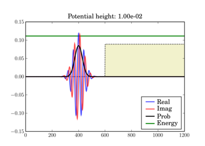
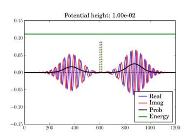
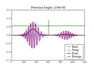
在这些图中,势以任意单位用黄色阴影表示,而波包的总能量以绿色线表示,单位与势相同。因此,虽然能量单位不是左侧轴上的单位,但两个能量图都使用相同的单位,因此可以有效地相互比较。
根据粒子的能量,黄色区域可能是经典禁区(当绿色线位于黄色区域内时)。
波包在 t=0 时开始(显示阶梯势)

在模拟结束时,它可能看起来像这样,具体取决于实际的势垒高度


这说明了根据势垒高度穿过薄势垒的隧穿。在第二种情况下,经典粒子将完全反弹,因为它的能量低于势垒。


代码
在 [1]
#=============================================================================
#
#               Quantum Mechanical Simulation using Finite-Difference
#               Time-Domain (FDTD) Method
#
#       This script simulates a probability wave in the presence of multiple
#       potentials.  The simulation is c arried out by using the FDTD algorithm
#       applied to the Schrodinger equation.  The program is intended to act as
#       a demonstration of the FDTD algorithm and can be used as an educational
#       aid for quantum mechanics and numerical methods.  The simulation
#       parameters are defined in the code constants and can be freely
#       manipulated to see different behaviors.
#
#       NOTES
#
#       The probability density plots are amplified by a factor for visual
#       purposes.  The psi_p quanity contains the actual probability density
#       without any rescaling.
#
#       BEWARE: The time step, dt, has strict requirements or else the
#       simulation becomes unstable.
#
#       The code has three built-in potential functions for demonstration.
#
#       1) Constant potential: Demonstrates a free particle with dispersion.
#
#       2) Step potential: Demonstrates transmission and reflection.
#
#       3) Potential barrier: Demonstrates tunneling.
#
#       By tweaking the height of the potential (V0 below) as well as the
#       barrier thickness (THCK below), you can see different behaviors: full
#       reflection with no noticeable transmission, transmission and
#       reflection, or mostly transmission with tunneling.
#
#               This script requires pylab and numpy to be installed with
#               Python or else it will not run.
#
#============================================================================
# Author:  James Nagel <nagel@mers.byu.edu>
#          5/25/07
#
# Updates by Fernando Perez <Fernando.Perez@colorado.edu>, 7/28/07
#============================================================================
#  Numerical and plotting libraries
import numpy as np
import pylab
# Set pylab to interactive mode so plots update when run outside ipython
pylab.ion()
#=============================================================================
# Utility functions
#  Defines a quick Gaussian pulse function to act as an envelope to the wave
#  function.
def Gaussian(x,t,sigma):
    """  A Gaussian curve.
        x = Variable
        t = time shift
        sigma = standard deviation      """
    return np.exp(-(x-t)**2/(2*sigma**2))
def free(npts):
    "Free particle."
    return np.zeros(npts)
def step(npts,v0):
    "Potential step"
    v = free(npts)
    v[npts/2:] = v0
    return v
def barrier(npts,v0,thickness):
    "Barrier potential"
    v = free(npts)
    v[npts/2:npts/2+thickness] = v0
    return v
def fillax(x,y,*args,**kw):
    """Fill the space between an array of y values and the x axis.
    All args/kwargs are passed to the pylab.fill function.
    Returns the value of the pylab.fill() call.
    """
    xx = np.concatenate((x,np.array([x[-1],x[0]],x.dtype)))
    yy = np.concatenate((y,np.zeros(2,y.dtype)))
    return pylab.fill(xx, yy, *args,**kw)

#=============================================================================
#
#  Simulation Constants.  Be sure to include decimal points on appropriate
#  variables so they become floats instead of integers.
#
N    = 1200     #  Number of spatial points.
T    = 5*N      #  Number of time steps.  5*N is a nice value for terminating
                #  before anything reaches the boundaries.
Tp   = 50       #  Number of time steps to increment before updating the plot.
dx   = 1.0e0    #  Spatial resolution
m    = 1.0e0    #  Particle mass
hbar = 1.0e0    #  Plank's constant
X    = dx*np.linspace(0,N,N)        #  Spatial axis.
# Potential parameters.  By playing with the type of potential and the height
# and thickness (for barriers), you'll see the various transmission/reflection
# regimes of quantum mechanical tunneling.
V0   = 1.0e-2   #  Potential amplitude (used for steps and barriers)
THCK = 15       # "Thickness" of the potential barrier (if appropriate
                # V-function is chosen)
# Uncomment the potential type you want to use here:
# Zero potential, packet propagates freely.
#POTENTIAL = 'free'
# Potential step.  The height (V0) of the potential chosen above will determine
# the amount of reflection/transmission you'll observe
POTENTIAL = 'step'
# Potential barrier.  Note that BOTH the potential height (V0) and thickness
# of the barrier (THCK) affect the amount of tunneling vs reflection you'll
# observe.
#POTENTIAL = 'barrier'
#  Initial wave function constants
sigma = 40.0 # Standard deviation on the Gaussian envelope (remember Heisenberg
             #  uncertainty).
x0 = round(N/2) - 5*sigma # Time shift
k0 = np.pi/20 # Wavenumber (note that energy is a function of k)
# Energy for a localized gaussian wavepacket interacting with a localized
# potential (so the interaction term can be neglected by computing the energy
# integral over a region where V=0)
E = (hbar**2/2.0/m)*(k0**2+0.5/sigma**2)
#=============================================================================
# Code begins
#
# You shouldn't need to change anything below unless you want to actually play
# with the numerical algorithm or modify the plotting.
#
#  Fill in the appropriate potential function (is there a Python equivalent to
#  the SWITCH statement?).
if POTENTIAL=='free':
    V = free(N)
elif POTENTIAL=='step':
    V = step(N,V0)
elif POTENTIAL=='barrier':
    V = barrier(N,V0,THCK)
else:
    raise ValueError("Unrecognized potential type: %s" % POTENTIAL)
#  More simulation parameters.  The maximum stable time step is a function of
#  the potential, V.
Vmax = V.max()            #  Maximum potential of the domain.
dt   = hbar/(2*hbar**2/(m*dx**2)+Vmax)         #  Critical time step.
c1   = hbar*dt/(m*dx**2)                       #  Constant coefficient 1.
c2   = 2*dt/hbar                               #  Constant coefficient 2.
c2V  = c2*V  # pre-compute outside of update loop
# Print summary info
print 'One-dimensional Schrodinger equation - time evolution'
print 'Wavepacket energy:   ',E
print 'Potential type:      ',POTENTIAL
print 'Potential height V0: ',V0
print 'Barrier thickness:   ',THCK
#  Wave functions.  Three states represent past, present, and future.
psi_r = np.zeros((3,N)) #  Real
psi_i = np.zeros((3,N)) #  Imaginary
psi_p = np.zeros(N,)   # Observable probability (magnitude-squared
                          #  of the complex wave function).
#  Temporal indexing constants, used for accessing rows of the wavefunctions.
PA = 0                 #  Past
PR = 1                 #  Present
FU = 2                 #  Future
#  Initialize wave function.  A present-only state will "split" with half the
#  wave function propagating to the left and the other half to the right.
#  Including a "past" state will cause it to propagate one way.
xn = range(1,N/2)
x = X[xn]/dx    #  Normalized position coordinate
gg = Gaussian(x,x0,sigma)
cx = np.cos(k0*x)
sx = np.sin(k0*x)
psi_r[PR,xn] = cx*gg
psi_i[PR,xn] = sx*gg
psi_r[PA,xn] = cx*gg
psi_i[PA,xn] = sx*gg
# Initial normalization of wavefunctions
#   Compute the observable probability.
psi_p = psi_r[PR]**2 + psi_i[PR]**2
#  Normalize the wave functions so that the total probability in the simulation
#  is equal to 1.
P   = dx * psi_p.sum()                      #  Total probability.
nrm = np.sqrt(P)
psi_r /= nrm
psi_i /= nrm
psi_p /= P
#  Initialize the figure and axes.
pylab.figure()
xmin = X.min()
xmax = X.max()
ymax = 1.5*(psi_r[PR]).max()
pylab.axis([xmin,xmax,-ymax,ymax])
#  Initialize the plots with their own line objects.  The figures plot MUCH
#  faster if you simply update the lines as opposed to redrawing the entire
#  figure.  For reference, include the potential function as well.
lineR, = pylab.plot(X,psi_r[PR],'b',alpha=0.7,label='Real')
lineI, = pylab.plot(X,psi_i[PR],'r',alpha=0.7,label='Imag')
lineP, = pylab.plot(X,6*psi_p,'k',label='Prob')
pylab.title('Potential height: %.2e' % V0)
# For non-zero potentials, plot them and shade the classically forbidden region
# in light red, as well as drawing a green line at the wavepacket's total
# energy, in the same units the potential is being plotted.
if Vmax !=0 :
    # Scaling factor for energies, so they fit in the same plot as the
    # wavefunctions
    Efac = ymax/2.0/Vmax
    V_plot = V*Efac
    pylab.plot(X,V_plot,':k',zorder=0)   #  Potential line.
    fillax(X,V_plot, facecolor='y', alpha=0.2,zorder=0)
    # Plot the wavefunction energy, in the same scale as the potential
    pylab.axhline(E*Efac,color='g',label='Energy',zorder=1)
pylab.legend(loc='lower right')
pylab.draw()
# I think there's a problem with pylab, because it resets the xlim after
# plotting the E line.  Fix it back manually.
pylab.xlim(xmin,xmax)
#  Direct index assignment is MUCH faster than using a spatial FOR loop, so
#  these constants are used in the update equations.  Remember that Python uses
#  zero-based indexing.
IDX1 = range(1,N-1)                            #  psi [ k ]
IDX2 = range(2,N)                              #  psi [ k + 1 ]
IDX3 = range(0,N-2)                            #  psi [ k - 1 ]
for t in range(T+1):
    # Precompute a couple of indexing constants, this speeds up the computation
    psi_rPR = psi_r[PR]
    psi_iPR = psi_i[PR]
    #  Apply the update equations.
    psi_i[FU,IDX1] = psi_i[PA,IDX1] + \
                      c1*(psi_rPR[IDX2] - 2*psi_rPR[IDX1] +
                          psi_rPR[IDX3])
    psi_i[FU] -= c2V*psi_r[PR]

    psi_r[FU,IDX1] = psi_r[PA,IDX1] - \
                      c1*(psi_iPR[IDX2] - 2*psi_iPR[IDX1] +
                          psi_iPR[IDX3])
    psi_r[FU] += c2V*psi_i[PR]
    #  Increment the time steps.  PR -> PA and FU -> PR
    psi_r[PA] = psi_rPR
    psi_r[PR] = psi_r[FU]
    psi_i[PA] = psi_iPR
    psi_i[PR] = psi_i[FU]
    #  Only plot after a few iterations to make the simulation run faster.
    if t % Tp == 0:
        #  Compute observable probability for the plot.
        psi_p = psi_r[PR]**2 + psi_i[PR]**2
        #  Update the plots.
        lineR.set_ydata(psi_r[PR])
        lineI.set_ydata(psi_i[PR])
        # Note: we plot the probability density amplified by a factor so it's a
        # bit easier to see.
        lineP.set_ydata(6*psi_p)

        pylab.draw()
# So the windows don't auto-close at the end if run outside ipython
pylab.ioff()
pylab.show()
部分作者:FernandoPerez、JamesNagel
附件